


1. INTRODUCTION
FMEA(Failure mode and effect analysis) is a powerful tool for system safety and reliability analysis of products and processes. FMEA is extensively used in a wide range of industries from manufacturing to service as examples of Sun et al.(2017), Apriliana et al.(2018), Fithri et al.(2018) and so on. In conventional FMEA, the risk of a failure or its cause is evaluated with RPN(Risk priority number), which is the mathematical product of its occurrence, severity and detection. Many authors discussed on the drawbacks of RPN and suggested alternative approaches for risk evaluation. Lieu et al.(2013) provided a literature review on risk evaluation approaches in FMEA up to 2013. Improvement efforts for RPN have been continued until recently, see Srivastava et al.(2018) for example.
Now AIAG(Automotive Industry Action Group) and VDA(German Association of the Automotive Industry) have been debating on their differences and making alignment for the 5thedition of FMEA handbooks(VDA QMC, 2018). Some important changes are i) FMEA-MSR (Monitoring and System Response) is added to maintain a safe state or a state of regulatory compliance during the client’s operation, ii) RPN is replaced by AP (Action Priority), iii) six steps of FMEA are specified, iv) the score tables are updated, and v) two types of recommended actions are to be provided, i.e. preventive action and detection action.
To determine priorities for preventive and detection action, FC(Failure Cause) should be more weighted than FM(Failure Mode). Considering the failure occurrence process, it should be noted that i) any failure occurs only after one of its causes occurs, ii) an FC detected before the actual failure does not induce failure, and iii) each FC has different frequency of occurrence and different inducing time of failure. But there are not so many works of FMEA that considers the role of time in the literature. Kwon et al.(2011), Kwon et al.(2013), Kwon et al.(2018), Jang et al.(2016), and Jang et al.(2016) are the few works which take account of time for risk evaluation in FMEA.
In this paper, we suggest a risk metric which may help determine AP for each FC. Assuming probabilistic models for failure and FC occurrences and detection, the risk metric is defined for FC. In Section 2, the failure occurrence process is described and a risk metric is defined for FC. Section 3 derives a formula to get the numerical value of the risk metric, assuming specific probability distributions. Section 4 provides a numerical example with some analyses and application to FMEA. And finally, some discussions and conclusion are followed.
2. THE RISK METRIC OF FC
Suppose the mission period (0, A] is given for the system. The risk of a failure cause is closely related with the severity and the occurrence process of the failure. If a failure actually occurs during the mission period (0, A], we may suffer some amount of losses. But we do not know exactly when will the failure occur and this uncertainty may cause additional expenses or costs. Thus, the risk may be supposed to have two components; i) the estimated loss due to the unfulfilled mission period and ii) the additional expense due to its uncertainty. Denote the failure time by a random variable T. Let μT and σT be the mean and standard deviation of T. Assuming a quadratic loss function, the risk due to the unfulfilled mission period may be evaluated as
where I(.) is an indicator function and a is a constant number unique to each FM. Note that each FM or FC will have different context of failure. And the time to failure will be different for each FC and FM. For fair comparison of the size of risk among different FC’s, the risk due to the uncertainty may be properly evaluated by
which is the coefficient of variation. Thus, we define the RFC (risk metric of FC) as
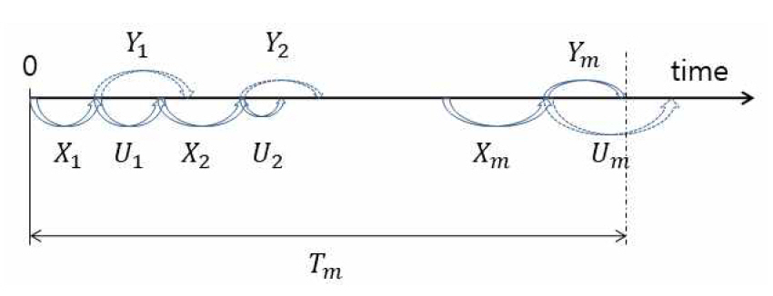
For convenience of deploy, we consider only one FC of an FM present, assuming the correction time of the FC is negligible. To get μT and σT, we should first examine the failure occurrence process. Let Xk be the kth occurrence time of the FC, Yk be the failure time due to the kth occurrence of the FC, and Uk be the detection time of the kth occurrence of the FC. If the number M of occurrence times of the FC before the actual failure occurs is given by m, the failure occurrence process can be depicted as Figure 1.
Note that the actual failure does not occur if the FC occurrence is detected and corrected before it occurs. Given M = m, the conditional failure time Tm can be expressed as
If we denote the probability mass function of M by p(m) and the probability density function of Tm by fTm(t), the probability density function of the actual failure time is obtained as
It may be impossible to get the closed functional form of fT(t). If the probability distributions of Xk, Yk and Uk are given, however, we can obtain μT and σT using the method of taking expectation of the conditional expectation like E[E(TM)]. And hence the size of risk can be evaluated.
3. NUMERICAL EVALUATION OF RFC
The distribution of T is not easy to derive even assuming simple distributions for Xk, Yk and Uk. In this section, we derive the specific formula of the risk metric (2) assuming exponential probability distributions for Xk, Yk and Uk. We further assume that X1, X2, ..., Xm are independently and identically distributed with the probability density function
Y1, Y2, ..., Ym are independently and identically distributed with the probability density function
and U1, U2, ..., Um are independently and identically distributed with the probability density function
3.1 The Mean and Variance of M
Before getting μT and σT, we should first derive the mean and variance of M. Since M is the number of occurrences of the FC until the actual failure occurs, it follows the geometric distribution with success probability
Thus, the probability mass function of M is given by
The mean and variance of M are
respectively.
3.2 The Mean and Variance of T
The distribution of T cannot be obtained as a closed form solution. So we first obtain the conditional mean and variance of T given M and then we get the mean and variance of T by taking the expectation of the conditional mean and variance. The conditional mean and variance of T given M = m are
respectively. And thus, the mean and variance of T are
respectively.
3.3 Validity of RFC
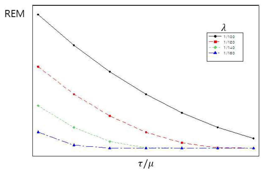
Using formula (1a), (1b), (2), (10a) and (10b), the risk metric can be evaluated quantitatively given the numerical values of λ, μ and τ. Both a and b are closely linked to the severity of FM, while λ, μ and τ are more related with FC. It will be worth examining the behavioral pattern of RFC against λ, μ and τ to confirm its validity. Figure 2 shows the graphs of REC versus τ/μ for λ = (1/100, 1/120, 1/140, 1/160).
Based on Figure 1, our intuition tells two general axioms; i) the risk will become smaller if λ takes smaller values and ii) the risk will decrease if τ/μ increases. Axiom i) says that if FC occurs rarely, then the failure risk will be small. And axiom ii) says that if FC is detected earlier before the actual failure occurs, the failure risk become smaller. Both axioms can be reasonably accepted.
Now if we look at Figure 2, the shape of RFC coincides with our intuitive axioms in most cases. When λ = 1/160, RFC has a slight increasing trend as increases. This may not be acceptable but it is a negligible quantity and hard to identify its increasing trend at all. When FC itself occurs very rarely i.e., λ takes very small value, the failure will not occur most of the time and the value of τ/μ does not make any meaningful difference. On the other hand, if τ/μ takes a very large value i.e., the FC is detected immediately upon its occurrence, the failure will not occur even if FC occurs frequently. Figure 2 seems to reflect these logical inferences very well. Thus, the RFC may be generally accepted as a good risk metric for FC.
4. APPLICATION TO FMEA
In this section, we take a numerical example to illustrate application to FMEA. We do not show the whole FMEA spreadsheets. Instead, we provide only relevant columns slightly modified to fit our purpose. And, for simplicity, we consider only one FM with several FC’s. A system or subsystem generally has many FM’s with many FC’s each. But the general situation can be handled similarly.
4.1 An Example
The main functions of the front door of an automobile are i) ingress to and egress from vehicle, ii) occupant protection from weather, noise, and side impact, iii) support anchorage for door hardware including mirror, hinges, latch and window regulator, iv) provide proper surface for appearance items, and v) paint and soft trim. Let’s consider the potential FM “Corroded interior lower door panels.” The potential effects of this FM are i) deteriorated life of door, ii) unsatisfactory appearance, and impaired function of interior door hardware. There are five possible FC’s with the values of λ, μ and τ shown in Table 1.
Considering the severity of the failure effects, suppose a = 1.0 and b = 0.5 is appropriate for this FM. And the mission period is 10 years. The numbers in the table are not real but fictional only for illustrative use.
Using formula (1a), (1b), (2), (10a) and (10b), we obtain the RFC values shown in Table 2. It is not surprising that the 6th FC “Insufficient room between panels for spray head access” has the biggest value of RFC and hence the first priority for action. It occurs the most frequently and cannot be detected effectively. Its detection probability before the occurrence of the actual failure is 1/(0.8+1) ≅ 0.56. The 3rd FC “Inappropriate wax formulation specified” occurs rarely with λ = 0.01 but it can be hardly detected, once it occurs, before the occurrence of the actual failure. Thus, its RFC value is close to other three FC’s of the 1st, 4th and 5th.
4.2 Sensitivity of μT, σ T 2
Note that μT and σ T 2 σ T 2
Figure 3 shows the pattern of change in μT against τ/μ. They shows linear positive relationship with steeper increment when λ is small. It is natural that μT increases as τ/μ increases and λ decreases. This implies that quicker detection and infrequent occurrence of FC prevents or delays the actual failure occurrence on the average.
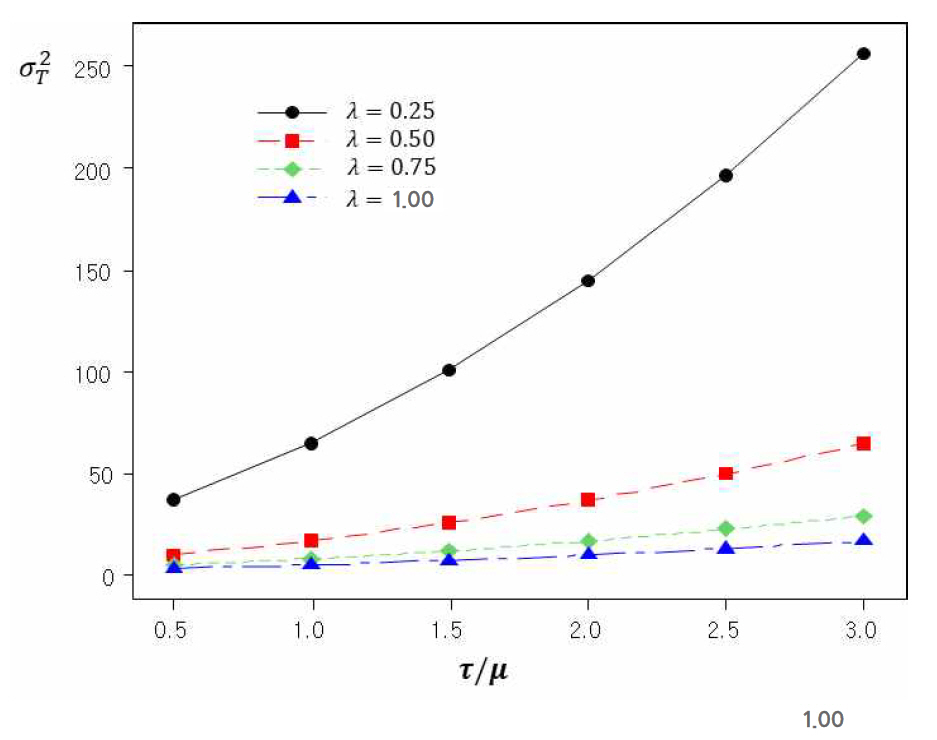
Figure 4 shows the pattern of change in σ T 2 σ T 2 σ T 2 σ T 2 σ T 2
Figure 5 shows the RFC curves against τ/μ. The actual failure will have smaller possibility to occur if FC occurs rarely and easily detected upon its occurrence. The RFC will have smaller values when λ is small and τ/μ gets bigger values. With a bigger value of λ, RFC tends to slowly decrease as τ/μ increases. But, with a smaller value of λ, RFC decreases more steeply at the early stage of increase in τ/μ.
5. DISCUSSIONS
In this section, we discuss some possible issues of the suggested risk metric RFC, which may need to be improved in future studies. We are sure that there should be many weak points better to be refined. But we discuss here only two points; i) about the definition of the risk metric and ii) about the assumptions on the distributions of failure occurrence and detection times.
5.1 Definition of the Risk Metric
To evaluate the risk related with failure in FMEA, Kwon et al.[7] employed three types of loss function; constant, linear and quadratic. And they proposed to use the expected loss for evaluation of the risk. For example, if we apply the quadratic loss function to our situation, the risk can be measured by
This is a simple and reasonable metric which is an acceptable and easily understandable concept. For practical use in the field application, however, the functional form of fT(t) cannot be derived, even with the most simple probability models for X, Y and U in (3). Thus, we cannot evaluate RFC of (11) even numerically. The only way to get a numerical value is using simulation. As a result of over tens of thousands calculations, we may obtain not an exact but an approximate value of the RFC.
This paper suggests a risk metric of (2) as an alternative to (11). Compared with (11), it may not be perfectly logical but it definitely is much simpler and may have a closed form solution, depending on situations. Moreover, it have some similar and reasonably acceptable characteristics.
5.2 Assumptions of the Probability Model
We assumed in this paper that all the probability models are exponential for X, Y and U in (3) for simplicity. But this is not a practical assumption. The exponential distribution may be appropriate for X but it usually is not appropriate for Y and U. Once an FC occurred, the failure is more likely to occur as time elapses. And detection may have similar properties. Thus, μ and τ are not constant anymore and increasing function of time.
Assuming the Weibull probability model for Y and U, μ(y) and τ(u) can be expressed as
respectively. Assuming the Weibull distributions with (12a) and (12b) for Y and U, we know their means and variances are
respectively, where Γ(.) is the gamma function. And μT and σ T 2
6. CONCLUSIONS
We proposed a risk metric for the failure cause in FMEA, which may possibly used as an alternative to RPN. The conventional metric RPN(risk priority number) has many drawbacks as discussed in many studies in the literature. The 5th edition of FMEA handbook also provides an improved metric.
We assumed that there are time gaps between the occurrence times of the failure cause and the failure itself. And also detection of a failure cause is assumed to require a length of time. Based on the assumed process of the failure and detection occurrence, we constructed a risk metric for a given failure cause. The metric can be calculated for any failure cause and thus can be used for determining AP(action priority) among all the failure causes in FMEA.
To use the proposed metric in FMEA, information on the failure and detection time distributions are necessary. But, in practical situations, it is very hard to get sufficient information necessary. Past experiences or knowledge of failure mechanism may be helpful in such situation. Sampling and life test data may also be necessary.
In future studies, practical cases or situations are expected over a wide range of industries where the time based model is applicable. Based on the real situations, the suggested model is open to modification, improvement or refinement.